Time Series Forecasting Project: Auto Sales and U.S. Monthly personal Income

Objective

Time-series models use a technique to extrapolate the historical behavior into the future. Figuratively, the series are being lifted into the future "by its own bootstraps." Time series data are historical in chronological order, with only one value per time period. This project aim s to use CB predictor to determine the best time series model used for predicting future value.

Variable and Measurements

CB predictor used eight different time-series modeling methods to obtain the best fit to the historical data series. CB predictor selects the best model based on the lowest Root Mean Square Error (RMSE) which resulted in the selection of the Holt-Winters Multiplicative model.

Mathematical Model

As mentioned earlier, CB predictor chose the best model of forecasting which is Holt- Winters Multiplicative.

Method ranking Table

	Method			RMSE	MAD	MAPE
Best: 	Holt-Winters' Multiplicative			63.8	47.386	3.61%
2nd:	Seasonal Multiplicative			66.237	50.329	3.83%
3rd:	Holt-Winters' Additive			69.381	52.092	4.09%
4th:	Seasonal Additive			70.657	53.532	4.19%
5th:	Double Moving Average			134.14	109.39	8.18%
6th:	Single Exponential Smoothing			136.1	109.38	8.43%
7th:	Single Moving Average			136.62	110.76	8.31%
8th:	Double Exponential Smoothing			137.59	111.41	8.68%

 RMSE (root mean square error) is an absolute error measure that square the deviations to keep the positive and negative deviations from canceling each other out.

MAD (Mean Absolute deviation): This an error that averages distance between each pair of actual and fitted data point.

MAPE (Mean absolute percentage error): this is a relative error measure that uses absolute values to keep the positive and negative errors from canceling each other  out and uses relative errors to let you compare forecast accuracy between time-series model.

Method Statistics: 					
						
		Method			Durbin-Watson	Theil's U
	Best: 	Holt-Winters' Multiplicative			2.019	0.429
	2nd:	Seasonal Multiplicative			2.001	0.449
	3rd:	Holt-Winters' Additive			1.993	0.458
	4th:	Seasonal Additive			2.011	0.468
	5th:	Double Moving Average			1.516	0.867
	6th:	Single Exponential Smoothing			2.014	0.943
	7th:	Single Moving Average			1.295	0.9
	8th:	Double Exponential Smoothing			2.025	0.942


	Method Parameters: 					
						
		Method			Parameter	Value
	Best: 	Holt-Winters' Multiplicative			Alpha	0.228
					Beta	0.001
					Gamma	0.001
	2nd:	Seasonal Multiplicative			Alpha	0.287
					Gamma	0.001
	3rd:	Holt-Winters' Additive			Alpha	0.291
					Beta	0.001
					Gamma	0.001
	4th:	Seasonal Additive			Alpha	0.335
					Gamma	0.001
	5th:	Double Moving Average			Periods	14
	6th:	Single Exponential Smoothing			Alpha	0.609
	7th:	Single Moving Average			Periods	14
	8th:	Double Exponential Smoothing			Alpha	0.627
					Beta	0.014

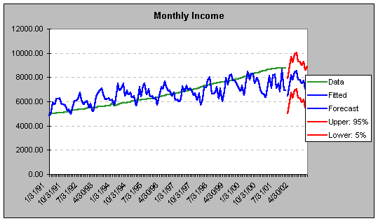
   The following graph shows a well fit between the projected data and the historical data.

Model Validity and Testing

Date                        Lower5% Forecast   Upper 95%

1/31/02		1117.20	1222.95	1328.70	
2/28/02		1278.44	1385.01	1491.57	
3/31/02		1540.69	1648.08	1755.48	
4/30/02		1435.56	1543.79	1652.02	
5/31/02		1587.04	1696.13	1805.21	
6/30/02		1610.97	1720.92	1830.87	
7/31/02		1429.86	1540.69	1651.52	
8/31/02		1430.43	1542.15	1653.88	
9/30/02		1360.88	1473.51	1586.14	
10/31/02		1414.92	1528.47		
11/30/02		1249.87	1364.36		
12/31/02		1317.43	1432.88	

Spreadsheet model